Introduction

Welcome to the world of Probability in Data Science! Let me start things off with an intuitive example.

Suppose you are a teacher at a university. After checking assignments for a week, you graded all the students. You gave these graded papers to a data entry guy in the university and tell him to create a spreadsheet containing the grades of all the students. But the guy only stores the grades and not the corresponding students.

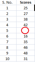
He made another blunder, he missed a couple of entries in a hurry and we have no idea whose grades are missing. Let’s find a way to solve this.

One way is that you visualize the grades and see if you can find a trend in the data.

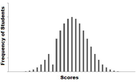
The graph that you have plot is called the frequency distribution of the data. You see that there is a smooth curve like structure that defines our data, but do you notice an anomaly? We have an abnormally low frequency at a particular score range. So the best guess would be to have missing values that remove the dent in the distribution.

This is how you would try to solve a real-life problem using data analysis. For any Data Scientist, a student or a practitioner, distribution is a must know concept. It provides the basis for analytics and inferential statistics.

While the concept of probability gives us the mathematical calculations, distributions help us actually visualize what’s happening underneath.

In this article, I have covered some important probability distributions which are explained in a lucid as well as comprehensive manner.

Note: This article assumes you have a basic knowledge of probability. If not, you can refer this probability distributions.

Table of Contents

1. Common Data Types
2. Types of Distributions
   1. Bernoulli Distribution
   2. Uniform Distribution
   3. Binomial Distribution
   4. Normal Distribution
   5. Poisson Distribution
   6. Exponential Distribution
3. Relations between the Distributions
4. Test your Knowledge!

Common Data Types

Before we jump on to the explanation of distributions, let’s see what kind of data can we encounter. The data can be discrete or continuous.

Discrete Data, as the name suggests, can take only specified values. For example, when you roll a die, the possible outcomes are 1, 2, 3, 4, 5 or 6 and not 1.5 or 2.45.

Continuous Data can take any value within a given range. The range may be finite or infinite. For example, A girl’s weight or height, the length of the road. The weight of a girl can be any value from 54 kgs, or 54.5 kgs, or 54.5436kgs.

Now let us start with the types of distributions.

Types of Distributions

Bernoulli Distribution

Let’s start with the easiest distribution that is Bernoulli Distribution. It is actually easier to understand than it sounds!

All you cricket junkies out there! At the beginning of any cricket match, how do you decide who is going to bat or ball? A toss! It all depends on whether you win or lose the toss, right? Let’s say if the toss results in a head, you win. Else, you lose. There’s no midway.

A Bernoulli distribution has only two possible outcomes, namely 1 (success) and 0 (failure), and a single trial. So the random variable X which has a Bernoulli distribution can take value 1 with the probability of success, say p, and the value 0 with the probability of failure, say q or 1-p.

Here, the occurrence of a head denotes success, and the occurrence of a tail denotes failure.
Probability of getting a head = 0.5 = Probability of getting a tail since there are only two possible outcomes.

The probability mass function is given by: p^x(1-p)^1-x  where x € (0, 1).
It can also be written as

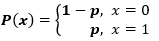
The probabilities of success and failure need not be equally likely, like the result of a fight between me and Undertaker. He is pretty much certain to win. So in this case probability of my success is 0.15 while my failure is 0.85

Here, the probability of success(p) is not same as the probability of failure. So, the chart below shows the Bernoulli Distribution of our fight.

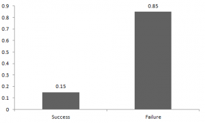
Here, the probability of success = 0.15 and probability of failure = 0.85. The expected value is exactly what it sounds. If I punch you, I may expect you to punch me back. Basically expected value of any distribution is the mean of the distribution. The expected value of a random variable X from a Bernoulli distribution is found as follows:

E(X) = 1*p + 0*(1-p) = p

The variance of a random variable from a bernoulli distribution is:

V(X) = E(X²) – [E(X)]² = p – p² = p(1-p)

There are many examples of Bernoulli distribution such as whether it’s going to rain tomorrow or not where rain denotes success and no rain denotes failure and Winning (success) or losing (failure) the game.

Uniform Distribution

When you roll a fair die, the outcomes are 1 to 6. The probabilities of getting these outcomes are equally likely and that is the basis of a uniform distribution. Unlike Bernoulli Distribution, all the n number of possible outcomes of a uniform distribution are equally likely.

A variable X is said to be uniformly distributed if the density function is:

The graph of a uniform distribution curve looks like

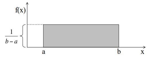
You can see that the shape of the Uniform distribution curve is rectangular, the reason why Uniform distribution is called rectangular distribution.

For a Uniform Distribution, a and b are the parameters. 

The number of bouquets sold daily at a flower shop is uniformly distributed with a maximum of 40 and a minimum of 10.

Let’s try calculating the probability that the daily sales will fall between 15 and 30.

The probability that daily sales will fall between 15 and 30 is (30-15)*(1/(40-10)) = 0.5

Similarly, the probability that daily sales are greater than 20 is  = 0.667

The mean and variance of X following a uniform distribution is:

Mean -> E(X) = (a+b)/2

Variance -> V(X) =  (b-a)²/12

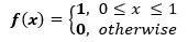
The standard uniform density has parameters a = 0 and b = 1, so the PDF for standard uniform density is given by:

Binomial Distribution

Let’s get back to cricket.  Suppose that you won the toss today and this indicates a successful event. You toss again but you lost this time. If you win a toss today, this does not necessitate that you will win the toss tomorrow. Let’s assign a random variable, say X, to the number of times you won the toss. What can be the possible value of X? It can be any number depending on the number of times you tossed a coin.

There are only two possible outcomes. Head denoting success and tail denoting failure. Therefore, probability of getting a head = 0.5 and the probability of failure can be easily computed as: q = 1- p = 0.5.

A distribution where only two outcomes are possible, such as success or failure, gain or loss, win or lose and where the probability of success and failure is same for all the trials is called a Binomial Distribution.

The outcomes need not be equally likely. Remember the example of a fight between me and Undertaker? So, if the probability of success in an experiment is 0.2 then the probability of failure can be easily computed as q = 1 – 0.2 = 0.8.

Each trial is independent since the outcome of the previous toss doesn’t determine or affect the outcome of the current toss. An experiment with only two possible outcomes repeated n number of times is called binomial. The parameters of a binomial distribution are n and p where n is the total number of trials and p is the probability of success in each trial.

On the basis of the above explanation, the properties of a Binomial Distribution are

1. Each trial is independent.
2. There are only two possible outcomes in a trial- either a success or a failure.
3. A total number of n identical trials are conducted.
4. The probability of success and failure is same for all trials. (Trials are identical.)

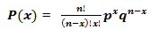
The mathematical representation of binomial distribution is given by:

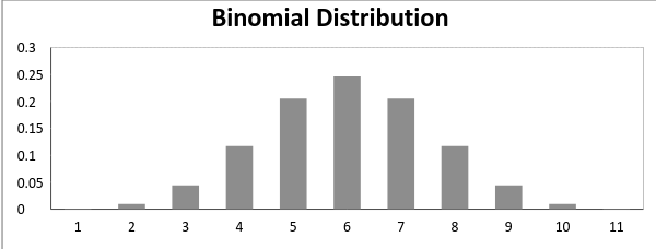
A binomial distribution graph where the probability of success does not equal the probability of failure looks like

Now, when probability of success = probability of failure, in such a situation the graph of binomial distribution looks like

The mean and variance of a binomial distribution are given by:

Mean -> µ = n*p

Variance -> Var(X) = n*p*q

Normal Distribution

Normal distribution represents the behavior of most of the situations in the universe (That is why it’s called a “normal” distribution. I guess!). The large sum of (small) random variables often turns out to be normally distributed, contributing to its widespread application. Any distribution is known as Normal distribution if it has the following characteristics:

1. The mean, median and mode of the distribution coincide.
2. The curve of the distribution is bell-shaped and symmetrical about the line x=μ.
3. The total area under the curve is 1.
4. Exactly half of the values are to the left of the center and the other half to the right.

A normal distribution is highly different from Binomial Distribution. However, if the number of trials approaches infinity then the shapes will be quite similar.

The PDF of a random variable X following a normal distribution is given by:

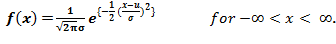
The mean and variance of a random variable X which is said to be normally distributed is given by:

Mean -> E(X) = µ

Variance -> Var(X) = σ^2

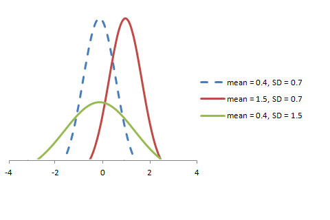
Here, µ (mean) and σ (standard deviation) are the parameters.
The graph of a random variable X ~ N (µ, σ) is shown below.

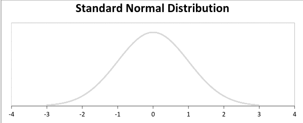
A standard normal distribution is defined as the distribution with mean 0 and standard deviation 1.  For such a case, the PDF becomes:

Poisson Distribution

Suppose you work at a call center, approximately how many calls do you get in a day? It can be any number. Now, the entire number of calls at a call center in a day is modeled by Poisson distribution. Some more examples are

1. The number of emergency calls recorded at a hospital in a day.
2. The number of thefts reported in an area on a day.
3. The number of customers arriving at a salon in an hour.
4. The number of suicides reported in a particular city.
5. The number of printing errors at each page of the book.

You can now think of many examples following the same course. Poisson Distribution is applicable in situations where events occur at random points of time and space wherein our interest lies only in the number of occurrences of the event.

A distribution is called Poisson distribution when the following assumptions are valid:

1. Any successful event should not influence the outcome of another successful event.
2. The probability of success over a short interval must equal the probability of success over a longer interval.
3. The probability of success in an interval approaches zero as the interval becomes smaller.

Now, if any distribution validates the above assumptions then it is a Poisson distribution. Some notations used in Poisson distribution are:

• λ is the rate at which an event occurs,
• t is the length of a time interval,
• And X is the number of events in that time interval.

Here, X is called a Poisson Random Variable and the probability distribution of X is called Poisson distribution.

Let µ denote the mean number of events in an interval of length t. Then, µ = λ*t.

The PMF of X following a Poisson distribution is given by:

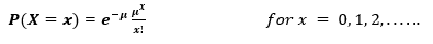
The mean µ is the parameter of this distribution. µ is also defined as the λ times length of that interval. The graph of a Poisson distribution is shown below:

The graph shown below illustrates the shift in the curve due to increase in mean.

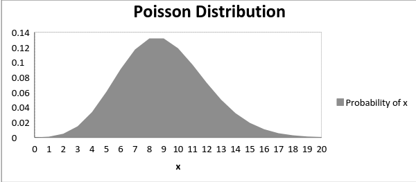
It is perceptible that as the mean increases, the curve shifts to the right.

The mean and variance of X following a Poisson distribution:

Mean -> E(X) = µ
Variance -> Var(X) = µ

Exponential Distribution

Let’s consider the call center example one more time. What about the interval of time between the calls ? Here, exponential distribution comes to our rescue. Exponential distribution models the interval of time between the calls.

Other examples are:

1. Length of time beteeen metro arrivals,
2. Length of time between arrivals at a gas station
3. The life of an Air Conditioner

Exponential distribution is widely used for survival analysis. From the expected life of a machine to the expected life of a human, exponential distribution successfully delivers the result.

A random variable X is said to have an exponential distribution with PDF:

f(x) = { λe^-λx,  x ≥ 0

and parameter λ>0 which is also called the rate.

For survival analysis, λ is called the failure rate of a device at any time t, given that it has survived up to t.

Mean and Variance of a random variable X following an exponential distribution:

Mean -> E(X) = 1/λ

Variance -> Var(X) = (1/λ)²

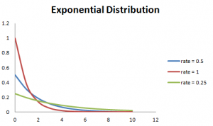
Also, the greater the rate, the faster the curve drops and the lower the rate, flatter the curve. This is explained better with the graph shown below.

To ease the computation, there are some formulas given below.
P{X≤x} = 1 – e^-λx, corresponds to the area under the density curve to the left of x.

P{X>x} = e^-λx, corresponds to the area under the density curve to the right of x.

P{x1<X≤ x2} = e^-λx1 – e^-λx2, corresponds to the area under the density curve between x1 and x2.

Relations between the Distributions

Relation between Bernoulli and Binomial Distribution

1. Bernoulli Distribution is a special case of Binomial Distribution with a single trial.

2. There are only two possible outcomes of a Bernoulli and Binomial distribution, namely success and failure.

3. Both Bernoulli and Binomial Distributions have independent trails.

Relation between Poisson and Binomial Distribution

Poisson Distribution is a limiting case of binomial distribution under the following conditions:

1. The number of trials is indefinitely large or n → ∞.
2. The probability of success for each trial is same and indefinitely small or p →0.
3. np = λ, is finite.

Relation between Normal and Binomial Distribution & Normal and Poisson Distribution:

Normal distribution is another limiting form of binomial distribution under the following conditions:

1. The number of trials is indefinitely large, n → ∞.
2. Both p and q are not indefinitely small.

The normal distribution is also a limiting case of Poisson distribution with the parameter λ →∞.

Relation between Exponential and Poisson Distribution:

If the times between random events follow exponential distribution with rate λ, then the total number of events in a time period of length t follows the Poisson distribution with parameter λt.

Test your knowledge

You have come this far. Now, are you able to answer the following questions? Let me know in the comments below!

1. The formula to calculate standard normal random variable is:

a. (x+µ) / σ
b. (x-µ) / σ
c. (x-σ) / µ

2. In Bernoulli Distribution, the formula for calculating standard deviation is given by:

a. p (1 – p)
b. SQRT(p(p – 1))
c. SQRT(p(1 – p))

3. For a normal distribution, an increase in the mean will:

a. shift the curve to the left
b. shift the curve to the right
c. flatten the curve

4. The lifetime of a battery is exponentially distributed with λ = 0.05 per hour. The probability for a battery to last between 10 and 15 hours is:

a.0.1341
b.0.1540
c.0.0079

End Notes

Probability Distributions are prevalent in many sectors, namely, insurance, physics, engineering, computer science and even social science wherein the students of psychology and medical are widely using probability distributions. It has an easy application and widespread use. This article highlighted six important distributions which are observed in day-to-day life and explained their application. Now you will be able to identify, relate and differentiate among these distributions.